This video is about the conceptual design of a Cryogenic Rocket Turbopump with CFturbo.
At first, you create a new project choosing the pump design module. Insert the design point of the pump. The design point, or duty point, is defined by volume flow rate, total pressure, and rotational speed. In this case, the fluid is Liquid Oxygen.
In CFturbo gases, liquids or mixtures can be specified using the CoolProp database. We have to specify the inlet conditions, and there are several options to define a pre-swirl, if applicable
On the right side, you’ll see the specific speed and the general machine type and some physical key values.
Now we add new components by starting CFturbos’ “stage designer”. In this example, we will design a dual-stage pump made of an axial inducer and a radial main impeller. Here we must select the energy distribution between the inducer and the impeller. Usually, the inducer brings 8% to 12% of the total energy rise.
We are ready start to do the detailed design of the inducer running sequentially through all different design steps.
CFturbo is driven by fundamental physical equations and numerous empirical correlations. These approximation functions are taken from textbooks, research papers, and own data. So, our code will be able to provide reasonable and detailed 3D-models of all Turbomachinery components.
After calculating and adjusting the impeller main dimensions, we are modifying the axial length of the impeller, defining the position of leading and trailing edges.
Now we shape the leading edge and the meridional contour of the impeller. The geometrical description of the hub will be transformed into an S-shaped curve, which is typical for many inducers.
Finally, we add a simplified thickness of the hub solid, in order to create a true geometrical solid later for export reasons.
All Bezier points can be modified numerically by changing numbers in the pop-up window.
Next, we are designing the blade properties. In this window, we define the number of blades as well as the blade shape, the blade thickness on leading, and on training edges.
On the right side of the window, we have a graphical representation of the velocity triangles.
There are several models implemented for a slip factor correlation. For pumps, the most common is the Guelich model for inducer. Using these parameters, blade angles on leading and trailing edges will be computed on every span.
Then a method must be selected to calculate the radial equilibrium from hub to a shroud. The meridional and circumferential velocity components can be adjusted to balance pressure and centrifugal forces. In many cases, it is useful to choose the “variable load” option that enables you to shift the blade loading from hub to shroud.
In the next design step, we do the meanline design, which determines the curvature of the blade between leading and trailing edges on every span. The wrap angle of the blade can be adjusted graphically or numerically. On the right side of the window, we have several diagrams to evaluate geometrical and physical properties, like relative velocity, blade loading, or static pressure.
In CFturbo, the user can choose between various methods of blade design. Currently we offer conformal mapping, direct modification of the beta-distribution, as well as the so-called “inverse design” method that is based on blade loading distribution.
In the final two design steps for the impeller, we make the blade profiling, blade thickness distribution, and we should round up the leading and the trailing edges.
Switching to our 3D Model view, we can see the hub and blades of the inducer as three-dimensional CAD geometry.
At this point we are ready to create the second component, which is our main pump impeller. As specified before, the radial impeller will provide 88% of the total hydraulic energy, in this example 158,4 bar total pressure rise.
In the parameter section, we again use empirical correlations to calculate the dimensions of the impeller. For this example, we show the work coefficient, which defines the impeller diameter, and the hydraulic efficiency functions.
All impeller dimensions can be adjusted manually if required. This will influence the geometry of the model for subsequent design steps.
On the right side of the window, you see important physical values, a meridional section, and the Cordier diagram.
In the meridional view, at first, we adjust the relative axial position of the main impeller an bring it close to the inducer.
Then we modify shape and position of the leading edge, as well as the general shape of hub and shroud contours and the axial length of the impeller.
As shown here, adjustments of the curves can be made intuitively by drag-and-drop of Bezier points. Alternatively each Bezier-point can be placed numerically which is essential for batch mode runs. Tangential transitions between curves can be set automatically, or manually by defining an angle.
On the right side of the window there are diagrams for area progression and curvature which can assist you shaping the meridional contour of the impeller.
A plot gives an indication about the meridional velocity magnitude within the impeller. The meridional velocity is calculated by a potential flow method.
To finish the meridional contour of the impeller we add hub and shroud solids. For example, we can split the curves or transform them into Bezier splines.
For demonstration purposes, w are choosing a simple model of the hub and shroud contour. This tool is very flexible for modeling detailed hub and shroud geometry. All Bezier points can be modified numerically by changing numbers in the pop-up window.
The description of hub and shroud contours will be part of the secondary flow path design which will be done later.
Hub and shroud solids, as well as blades can be exported later into any CAD-format or meshing tool for FEA analysis.
Now we have to calculate the velocity triangle in the blade properties design window. In this window we define the number of blades as well as the blade shape, the blade thickness on leading and on training edges.
We chose 8 baldes, and the blade shape will remain on “freeform 3D” as recommended for such type of impellers.
There are several models implemented for a slip factor correlation. For pumps, the most common is the Guelich Wiesner [goolish wiesner] model, or the Pfleiderer correlation, that will be used here. Using these parameters, blade angles on leading and trailing edges will be computed on every span, like it was done for the inducer.
On the right side of the window we have a graphical and numerical representation of the velocity triangles and the slip factor correlation diagram, among others.
In the next design step, we do the meanline design which determines the curvature of the blade between leading and trailing edges on every span.
The wrap angle of the blade can be adjusted graphically or numerically. On the right side of the window, we have several diagrams to evaluate geometrical and physical properties.
You can see plots and diagrams for relative and absolute velocity, pressure, swirl, and blade loading, among others. These calculations are based on “Stanitz-Prian” methodology.
The user can choose between several different design modes for meanline design like conformal mapping or blade loading definition.
To finalize the geometry of the main impeller, in this case we just accept, the internal design proposals in the blade profile section, which uses a constant thickness for the blades.
Leading edges are given an elliptic shape, and the trailing edges will be left blunt and trimmed on the outer impeller diameter.
Now we can see both components, the inducer, and the main radial impeller, in our 3D-viewer.
On the left side of the window, there is a model tree showing components and sub-components which allow easy navigation, renaming as well as adjusting color and translucency.
A so-called “model finishing” enables the user to create and to export high-quality CAD-solid models for export. During the model finishing process, a user has the possibility to specify fillets on hub and shroud, if applicable.
Compared to other conceptual Turbomachinery design tools, CFturbo allows a very detailed geometry representation of all significant components.
This is an advantage for direct export to CFD- or FEA-codes without applying another 3D-CAD-system to prepare the computational domain.
Before we go ahead, we initially save the file.
At this point, we are ready to create the next component, which will be an un-vaned diffuser downstream of the impeller.
There are several different possibilities to define the general shape of the diffuser. Here we choose the radial diffuser option to create an initial geometry. Then we have the possibility to modify the length and the width of the diffuser by changing the numbers. We can put in relative or absolute values.
On the right side, we can see a meridional sketch of the diffuser, showing its position in a z-r-diagram.
In general, the Stator-module of CFturbo can be used to design either un-vaned diffusers or vaned, and return channels of high complexity including 2D- or -3D-shaped blades. like bowl diffusers for mixed-flow type machines.
The next component we design will be the volute. For volute design, we can select different cross-sections like round, radius based, freeform, etc. all symmetric and asymmetric. The cross-section shape can vary in the circumferential direction as well.
There are different velocity-based design rules to calculate the extension of the spiral, for example, the user can select between Pfleiderer- or Stepanoff- equations. Additionally, the user can create a spiral shape by their own geometrical requirements using the so-called geometry-based design mode. A correction factor can consider the influence of the cutwater thickness to the spiral shape.
Once the spiral contour is done, we make the discharge diffuser. We can specify the length and outlet diameter. There are different shapes available, and the discharge diffuser can be curved in axial direction too.
Finally, we create a fillet radius which represents the cutwater of the volute. Besides the fillet cutwater option, the user could go for so-called “simple” or “sharp” cutwater design.
Here the volute model is shown in the 3D viewer, besides the inducer and main impeller.
Since the 3D-viewer of CFturbo runs on a 3D-CAD-kernel, there are a large variety of display options, and numerous functions to create, to show and and to check the geometry models. This fundamental functionality is beneficial later when it comes to CAD-export and batch mode runs.
Again, now we rename components, and we change the transparency of the volute within the model tree on the left side of the screen.
On the right side of the window, informational comments and warnings are shown, which support the user in his design work. The comments are linked to an integrated online help manual.
To prepare a CFD model, the user should add a pipe on the suction side of the impeller. For this purpose, we add an axial stator.
The non-rotating component should be given a certain length, and there must be a small gap between pipe and impeller in order to create the secondary flow path later.
In this case, we have added a 100 mm pipe at the inlet, and a 2 mm gap between pipe and impeller.
Additionally, we have added a rounded hub nose contour in front of the inducer, to ensure an undisturbed inflow to this component. Its length, shape, and tangential transition can be exactly defined.
Later, when preparing the CFD-solver-set-up, the hub nose should be given the boundary condition “rotating wall”
The hub nose could get an arbitrary axis-symetric shape. We immediately can see the extended model in 3D. To finish this component design we rename the pipe on the inlet side as well.
To get a “water-tight” CAD model we are creating the secondary flow path which describes the space around the impeller.
In the current CFturbo version, the user has to add a tiny component between the two impellers to fulfill the internal requirements for secondary flow path design.
Another precondition making the secondary flow path is the creation of the hub and shroud solids. The initial secondary flow path describes a (more or less) simplified space which can be adjusted by drag-and-drop of Bezier points.
In general, there’s high flexibility in shaping the space between the impeller and the casing. The corner points can be adjusted graphically or numerically.
As shown here, the casing contours of the secondary flow region are created and are modified interactively. We split curves to place cornerpoints. All straight lines can be transformed into Bezier splines, if required.
One of the the advantages, to create the secondary flow path directly inin CFturbo, will be the ability to proceed with 3D-CAD-export and meshing without the incorporation of a third party CAD-system. This steamlines the whole CAE-process of design exploration and simulation. The rotational surfaces of the secondary flow regions can be modeled very detailed.
For example, here we modify the casing contour near the eye of the impeller. This is very often used to design a small gap to minimize volumetric losses. In general, the shroud contour of the impeller can be adjusted accordingly. The user could model a wear-ring, or a simplified labyrinth seal to prepare the CFD- geometry in already within CFturbo.
The user could model a wear-ring, or a simplified labyrinth seal to prepare the CFD-geometry in already within CFturbo.
Now we see the fully closed flow domain in our 3D viewer. Our model is ready for geometry export and simulation.
We change colors and repeat the model finishing for inducer and main radial impeller.
CFturbo has export formats to all major CFD-codes and CAD-systems, as well as neutral formats like STEP, STL, or Parasolid.
We always recommend 3D-CFD-simulations to evaluate pump geometry models designed in CFturbo. According to our experience, potential flow calculations, throughflow simulations or loss model based performance curve estimations will not be sufficient for a reliable feedback.
For Turbomachinery CFD-simulation codes like ANSYS-CFX, FINE/Turbo, StarCCM+, Simerics MP or TCFD allow cost-effective, accurate predictions of performance, hydraulic efficiency, shaft power, torque, NPSH and cavitation in general.
Another possibility would be export geometry components to create physical prototypes. Rapid prototyping methods allow to produce detailed and durable test models for many applications, but not for all kind of rotating machinery operating conditions.
Slide 1. As shown in this image, CFturbo has interfaces to various CFD-codes. All interfaces are under continuous improvement. The list will be extended if new codes enter the market.
Slide 2. Furthermore, it is essential to create robust, automated workflows that allow user-friendly access for experts and beginners. For CFturbo, there is a bi-directional integration into ANSYS Workbench available.
Slide 3. In recent years it has become more and more affordable to combine Turbomachinery design software and CFD-codes with optimization algorithms due to lower computational cost. Here we see an example for such a process combining CFturbo, ANSYS optiSlang, and Simerics MP. The rocket turbopump example had been exported to SimericsMP to run a CFD-simulation.
Slide4. Simerics MP is a modern, robust, fast, accurate, and cost-effective general-purpose 3D-Navier-Stokes-code. CFD-simulations with Simerics MP provide realistic results that compare accurately with multiple field tests.
Here we see a screenshot of a converged solution for the steady-state simulation using Simerics MP. Besides residuals, we’re able to monitor physical properties and integral values like head rise, hydraulic efficiency, shaft power, and torque.
This steady-state simulation on a three-million-nodes mesh took about thirty minutes on a laptop with an Intel I-7 processor. Transient simulations with four revolutions would take less than two hours to converge for the same model.
Final Slide cfturbo.com – get a free trial.