Background

Nonlinearity and Hysteresis definitions were developed to characterize performance of common sensors such as scales and load cells. Those definitions are widely used to characterize Torquemeters. Despite the similarities between Torquemeters and modern weighing devices, there are significant differences between them and their applications. Most important, real-world Torque signals are invariably dynamic whereas weighing, and most load measurements, are primarily static.

Thus, when those definitions are applied to Torquemeters, the results can be misleading, and, the conclusions based on them, wrong. This note describes traditional definitions as well as others that more accurately characterize real-world performance of Rotating and Reaction Torquemeters, used under dynamic conditions. It includes definitions, now used by Himmelstein, which provide the basis for valid product comparisons. It also discusses the impact Nonlinearity, Hysteresis and Overrange have on accuracy. Static characteristics such as temperature effects are valid for all common sensors and are not covered.

Nonlinearity

To avoid errors, a Torquemeter’s output must faithfully reflect its input. When it is nonlinear, its output contains errors in the average torque as well as its dynamic components (inevitably present on drivelines and other dynamic applications; see Himmelstein Application Note 221101D). Nonlinearity also generates output frequencies not present in the input torque. They include harmonics of the input frequency(s), and sum and difference frequencies; see Appendix 1. This situation is exacerbated during transient conditions. The only way to avoid such errors is to use a Torquemeter with minimal, correctly characterized, Nonlinearity, Hysteresis and Overrange.

Using a computer or microprocessor-based signal conditioner, it’s possible to “linearize” the calibration stand response of a nonlinear torquemeter. However, this procedure is only valid when the torque signal is static, i.e. has no sinusoidal components, perturbations, torque reversals, inertia torques, etc. – that’s never the case for a Rotating or other dynamic torque measurement, see Application Note 221101D. Although “linearization” can yield a very linear response on a calibration stand, it will produce significant additional errors in real-world, dynamic applications. The reported average torque will be in error and frequencies not present in the input signal, including harmonics of the input torque frequencies and sum and difference frequencies, will be generated; see Appendix 1.

Using a “linearizer” for a dynamic torque signal processes the distorted signal through another non-linear element. Not only can it not remove the signal’s distortion components, but, it increases their number. Beware of a Torquemeter that includes linearization software. While it can improve the linearity of a static calibration, it will generate additional errors in dynamic, “real world” applications.

To determine a Torquemeter’s Nonlinearity, one applies ascending and descending loads (usually 10 CW and 10 CCW) from a low uncertainty, Accredited Torque Calibration Stand and records the outputs. Nonlinearity is defined as the output’s greatest deviation of ascending data from a reference line that emulates the Torquemeter’s ascending response. It is expressed as a percentage of full scale.

The reference line often includes the end point but, it can intercept any one, two or no calibration points. When it includes the end point, the result is called End Point Nonlinearity. End Point Nonlinearity is simple to evaluate even without a computer. However, a line through the end point, or any other point is arbitrary and virtually never best characterizes the Torquemeter. As a result, when using the End Point, the sensor’s reported Nonlinearity is invariably different than its true Nonlinearity. A more accurate Nonlinearity is obtained by using a Least Squares Reference Line.

In summary, the output of any real world Torquemeter will deviate from a straight line. Conventionally, the output’s deviation from a Reference Line is determined for each ascending load point. Device Nonlinearity is defined as the greatest difference between the Torquemeter’s ascending output and the Reference Line. The Reference Line can be End Point, Zero Point, Least Squares, or others. Each of those Reference Line types will produce a different result. Therefore it is critically important to know which is used and its limitations when comparing or evaluating published linearity specifications.

Hysteresis

During calibration, the difference between the ascending and descending outputs at each load point is also calculated. Hysteresis is defined as the greatest difference between those values. It is expressed as a percent of full scale. Hysteresis is separately determined for CW and CCW torque directions. A Torquemeter’s Hysteresis is the greater of its CW and CCW values.

A Torquemeter will never see an error equal to Hysteresis as defined above. The Hysteresis error it sees is the deviation from the Reference Line, not the difference between ascending and descending values. Furthermore, in the conventional definition of Nonlinearity, the descending response is ignored. Because virtually all torque measurements are dynamic and include torque oscillations and reversals, the descending part of the response curve must be included to accurately depict Torquemeter performance including Hysteresis effects.

Combined Linearity and Hysteresis

A practical solution is to calculate the actual Error Band (EB), as follows. All ascending and descending calibration data is used to compute a Best-Fit Reference Line (BFL) for both CW and CCW directions. Then the greatest deviation from the BFL is found for CW and CCW loadings. The Torquemeters’ Combined Nonlinearity and Hysteresis is the greater of the CW and CCW deviations. This method has the advantage of accounting for ascending and descending response while intrinsically accounting for Hysteresis. Himmelstein now uses this definition for specifying and evaluating all its Torquemeter products. Not only does it realistically account for both ascending and descending data, but the reference BFL is based on all calibration steps (usually 21) and most closely matches the transducer.

Although more difficult to compute, a Best Fit Line (BFL) minimizes the difference between it and every ascending and descending calibration step. No other Reference Line can more accurately characterize a Torquemeter.

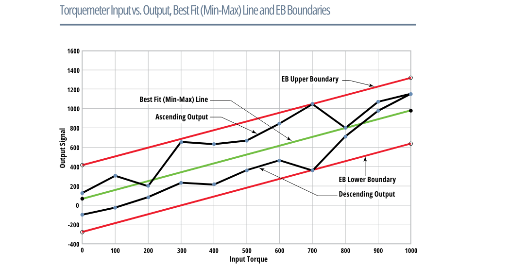
The diagram shown below is a typical calibration curve greatly exaggerated for clarity. It includes ascending and descending data, a Best Fit Reference line, and Error Band (EB) boundaries. When derived in this manner the Combined Error is conservative, i.e. the actual error is less than the error boundary values for all loads, except the two at the maximum error point(s).

Overrange

Unless a Torquemeter has adequate Overrange it will clip dynamic torque peaks in the upper part of its range. When that happens its output will contain additional large errors and its distortion components will be greatly magnified. All Himmelstein Digitally-based Torquemeters have between 150% and 300% Overrange, model dependent. Typical Combined Error in the Overrange region is 0.04%, maximum Combined Error is 0.1%. See Himmelstein Application Note 20805B for more information on the critical importance of Torquemeter Overrange.

Illustrative Examples

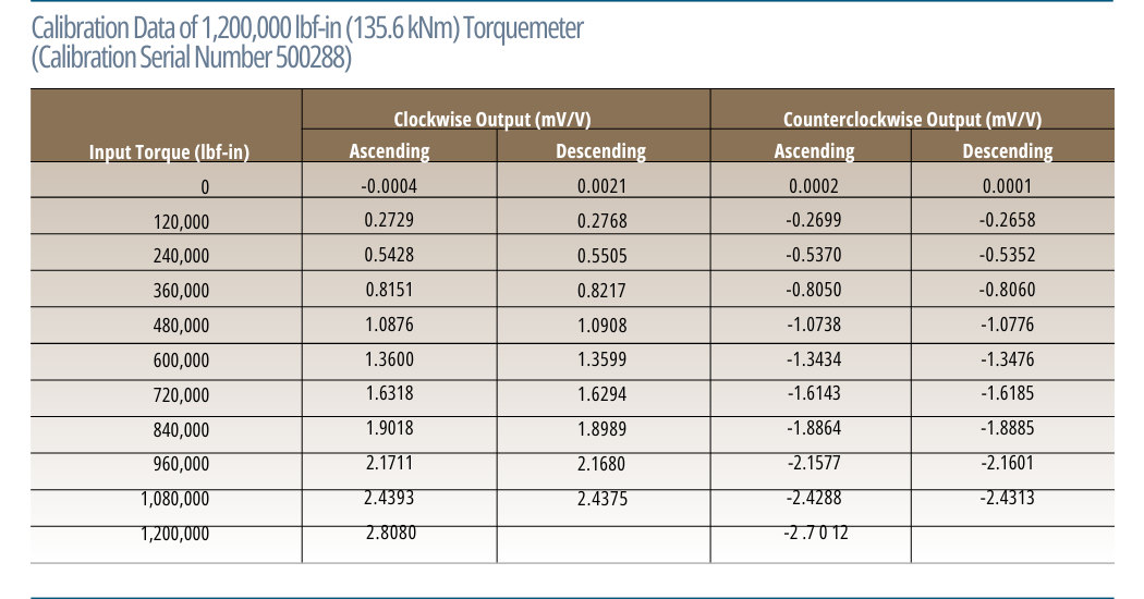
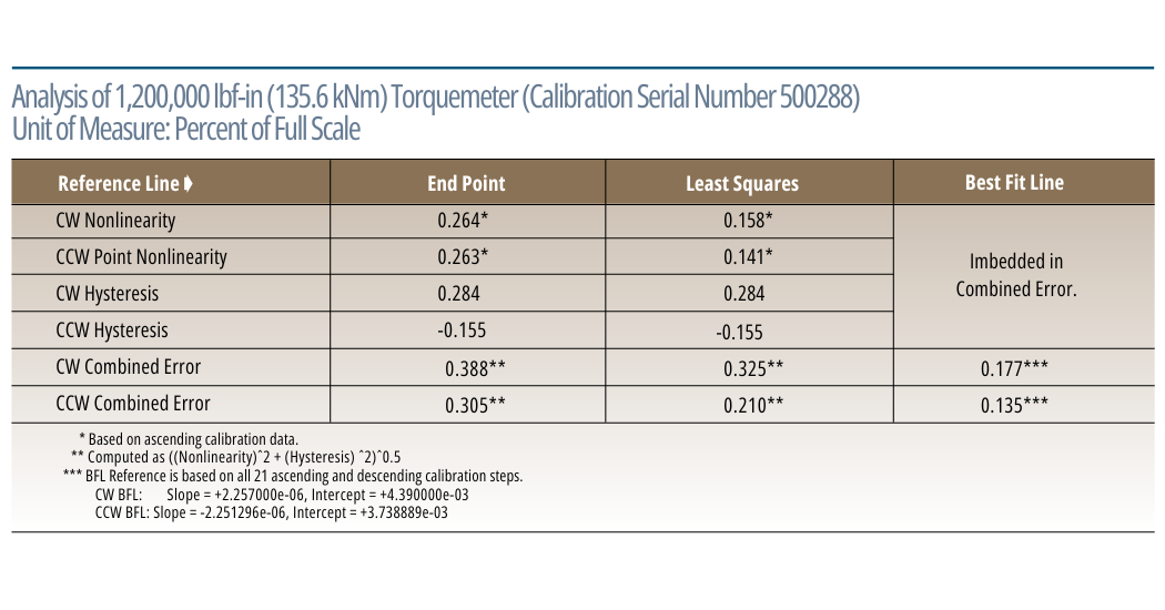
The first table summarizes the calibration of a non-Himmelstein Torquemeter performed in our laboratory. The next compares results using reference lines based on End Point, Least Squares and Best Fit Line. It shows significant differences in Nonlinearity and Combined Error when analyzed with different reference lines. When classifying modestly accurate Torquemeters such as this, valid performance evaluations and or comparisons can only be made when the most precise analysis method is used. In any case, you should know and understand the analysis method used and its limitations.

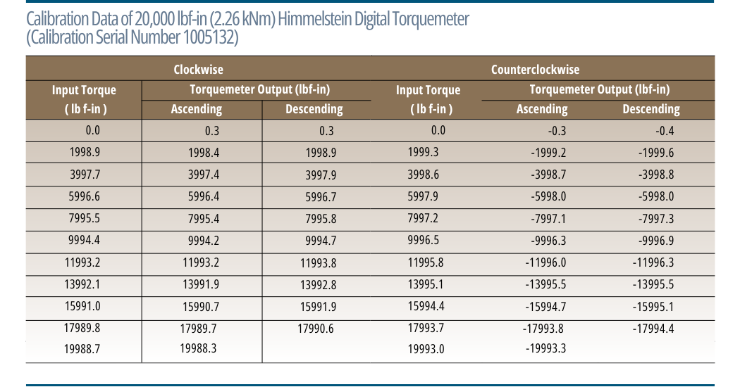
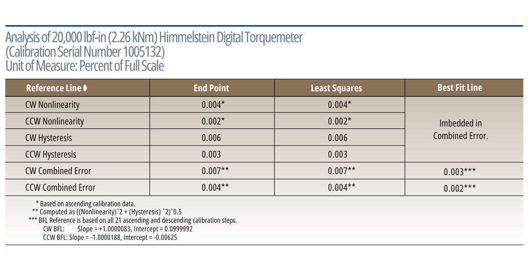
The next table contains calibration data of a very accurate Himmelstein Digital Torquemeter; Model MCRT 84004V(2-4) JOB. The last table summarizes its performance based on different analysis methods. High precision devices yield virtually identical results when analyzed with each method. If a Torquemeter were perfect, then all analysis methods will produce the same result, i.e., Nonlinearity, Hysteresis and Combined Error equal to zero. Nonetheless, the most accurate results will be achieved with the Best Fit Line method described above.

Appendix 1

How Nonlinearity Creates Amplitude Errors and Erroneous, Nonexistent Signals

A properly functioning Torquemeter’s response curve is smooth, and without gaps. If that isn’t the case, it is defective and should be repaired or replaced. Accordingly, a properly functioning Torquemeter’s response can be described by the following power series.

Output = a0 + a1Tin + a2Tin 2 + a3Tin 3 + a4Tin 4 + a5Tin 5 + (1)

Where a0, a1, a2 etc. are constant coefficients and Tin is the input Torque.

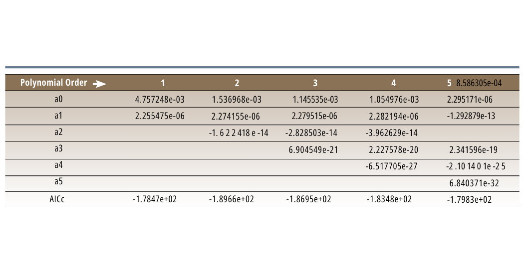
If the Torquemeter is perfectly linear, then its response is described by the first two terms. The following table contains the coefficients for equations of the 1st through 5th order. It is based on least square calculations that include both the ascending and descending CW response of the 1,200,000 lbf-in Torquemeter previously discussed. Also included is the Akaike Info Criterion (AICc); the best model has the lowest AICc.

Based on the Akaike Info Criterion, it’s clear the 2nd order equation is the best model for this Torquemeter. Therefore, for this analysis, we will use the 2nd order response. Further assume the dynamic input has an average value and two sinusoidal components. Thus, the input signal is:

Tin = Ta + Tb (sin ωb t) + Tc (sin ωc t)

Where Ta is the average value of the input torque and Tb is the peak amplitude of the sinusoidal component whose angular velocity is ωb. Similarly, Tc is the peak amplitude of the sinusoidal component whose angular velocity is ωc. If the Torquemeter were perfectly linear, it would output a scaled, mirror image of the input. That is, an average value directly proportional to Ta, a sine wave with ωb angular velocity and amplitude directly proportional to Tb and another with ωc angular velocity and amplitude directly proportional to Tc. The following steps show what is actually output.

The Torquemeter Output = a0 + a1Tin + a2Tin 2

Substituting Tin in the Output equation, yields

Output = a0 + a1[Ta + Tb (sin ωb t) + Tc (sin ωc t)] + a2[ Ta + Tb (sin ωb t) + Tc (sin ωc t)]2

Simplifying and using trigonometric identities for (sin ωt)2 and (sin ωb t) (sin ωc t ) yields: 9 terms. An average value (dc) term with error components, the two original sinusoidal terms with the correct amplitude proportionality, those same sinusoids with distorted amplitude proportionality, the second harmonic of each input sinusoid, and sinusoids whose frequencies are the sum and difference of the input signal frequencies. The exact output responses are listed below.

a0 + a1Ta + a2Ta 2 + a2Tb 2/2 + a2Tc 2/2 (average torque term. a0 can be zeroed out, a1Ta is the correct average torque output. The other terms are erroneous and cannot be corrected because they include unknown dynamic signal amplitudes)

+ a1 Tc (sin ωc t) + 2 a2 Ta Tc (sin ωc t) (ωc sinusoidal terms. 1st term is correct, the 2nd is an error component that cannot be corrected because it includes unknown dynamic signal amplitudes.)

+ a1 Tb (sin ωb t) + 2 a2 Ta Tb (sin ωb t) (ωb sinusoidal terms. 1st term is correct, the 2 nd is an error component.)

– a2 Tb 2(cos 2ωb t)/2 (2nd harmonic of ωb . This is an error term not present in the signal.)

– a2 Tc 2(cos 2ωc t)/2 (2nd harmonic of ωc . This is an error term not present in the signal.)

+ a2 Tb Tc (cos (ωb – ωc) t) – a2 Tb Tc (cos ( ωb + ωc ) t) (sum and difference frequencies, both are error components not present in the signal.)

Thus, the output contains error components added to the correct average value, error components added to both sinusoidal inputs, and sinusoids not in the input signal including second harmonics and sum and difference frequencies.

When more than two signal frequencies are present, additional sum and difference frequencies and harmonics will be output. If only a single signal frequency is present, errors will be generated in the average value, in the amplitude of the signal frequency, and a second harmonic of that frequency will be created.

When the devices Nonlinearity requires higher order terms to accurately represent it then, the number of distortion components increases. For example, when a third order term is required, a third harmonic of each sinusoid is generated –- sin 3 (ωt) = 1/4 (3 sin (ωt) – sin (3 ωt)). To avoid such errors, the Torquemeter must have an inherently linear response. “Linearizing” its response does not eliminate these errors, it compounds them.