Author: Ben Keiser, Applied Flow Technology
Piping and pumping systems are all around us. After all, transferring fluid from one point to another is what makes the world go ‘round right?
As engineers know, assuming a piping system is flat makes the fluid dynamic equations much easier to solve by neglecting elevation change. However, piping systems travel side to side, up and down, all over the place. So, with all the zigging and zagging associated with piping systems, elevation must be taken into account for the fluid dynamic equations to accurately predict system pressures and flow rates.
AFT works with a variety of industries, including the mining industry, to ensure models and simulations include accurate elevation changes. Piping systems for mining applications deal with significant elevation changes for slurry pipelines, mine dewatering, and leach pad operations. AFT Fathom and AFT Impulse can be used to easily solve the mathematical equations that dictate if these fluid transfer systems will function properly and of course, elevation data is required.
If you have elevation profile data, here are some tricks you can use to easily incorporate input data for a flow model in order to:
- Model systems where elevation changes are significant.
- Learn about previously unknown components after the model was built.
When you model your system, a lot of elevation changes require more pipes and components on the Workspace that clutter the model simply for the sake of accounting for elevation change. If a new component needs to be added to the middle of an existing model, one way to add a component would be to break the pipe connections, add the new junction, then draw and specify the additional pipes
AFT has features that will remove confusion and make modeling much easier! I’m going to address the elevation topic first.
Pipe elevation changes are necessary to properly calculate the pressures and flow rates of a piping system. Hydrostatics make an impact, and to assume there are no elevation changes is not the greatest idea. The way you consider piping elevation changes in AFT software is to specify the elevation input information into the junctions in the model.
The system below in Figure 1 demonstrates using junctions in a long pipeline to characterize elevation change. In my model, I have used the simple “Branch Junction” to enter the elevation at each point in the flow path. By default, the Branch Junctions are lossless.
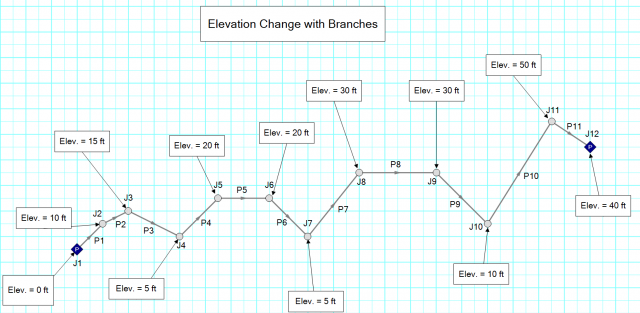
Figure 1 – Using Branch Junctions to characterize elevation changes.
In reality you have elbows, area changes, valves, and other types of fittings. You can lump minor losses due to pipe fittings into pipes as “Additional Fittings & Losses”. This blog here talks about how to simplify your model to include the effect of minor losses without cluttering the model with several junctions and short pipes. For this discussion, I’m will focus on elevation changes and neglecting minor losses.
In my model, I assigned an arbitrary length scale to my grid. One square in the X-direction is equal to 25 feet (7.62 meters) while one square in the Y-direction is equal to 5 feet (1.524 meters). Based upon the model layout on the grid, I was able to easily calculate the total length of each individual pipe segment, shown in Table 1.
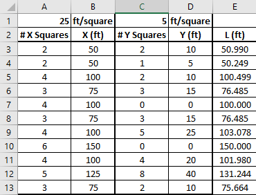
Table 1 – Horizontal & vertical lengths based on arbitrarily defined grid scaling. Total segment length in Column “E”.
There is a much easier way to account for all these elevation changes rather than having to use junctions like in Figure 1. In Figure 2, I only drew a single pipe from the inlet of the pipeline (J100) to the outlet (J101). Figure 3 shows how you can add multiple segments to a pipe from the Arrange menu, that way a single pipe can be drawn to look like that shown in Figure 2. You can add up to 25 segments in a single pipe and if you select a pipe and press “Control + Y” on your keyboard, this is another quick way to create the graphical pipe segments.
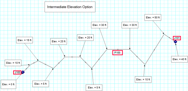
Figure 2 – Pipeline drawn with ten (10) intermediate pipe segments using the Pipe Segment tool from the Arrange menu.
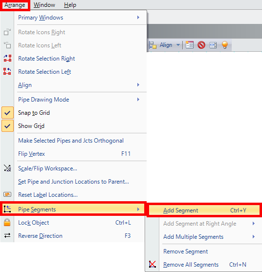
Figure 3 – Pipe Segment tool found from the Arrange menu.
In my single pipe, I created 10 intermediate points with the segmenting tool. If you count all the elevation Annotations and exclude the inlet (J100) and outlet (J101), you will see that there are 10 points. The Workspace illustrates the elevation profile with the annotations and segments I used, but the actual intermediate point elevation input is specified on the Optional tab of the Pipe Property window.
Opening the Pipe Property window allows you to specify the pipe characteristics. The length in this pipe is 1,016.675 feet (310 meters). The Optional tab is where you would check the box to “Use Intermediate Pipe Elevations” and then specify the Number of Intermediate Elevation Points, as shown in Figure 4. As mentioned previously, I have 10 intermediate points excluding the inlet and outlet of the system. Therefore, I would choose to use 10 Intermediate Elevations.
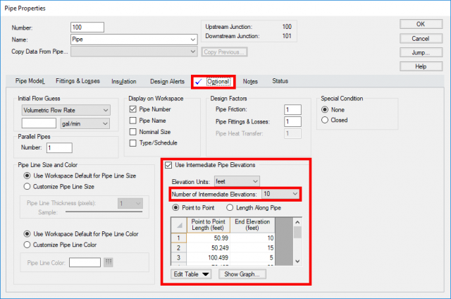
Figure 4 – Using 10 Intermediate Pipe Elevation points on the Optional tab of the Pipe Property window.
Now, this has been a feature that has existed in AFT software for a long time. However, there was only one option and that was to specify the Intermediate Elevation Changes in terms of the total Length Along the Pipe. In the latest version of AFT software (AFT Fathom 10, AFT Arrow 7, and soon AFT Impulse 7), there is a new choice available and this is to simply specify the individual length from point to point. This is much easier because as you are calculating the length in the pipe from your drawings, you do not have to keep track of the cumulative length along the pipe anymore. Table 2 includes the raw data from Table 1 and demonstrates how you can create a table that can easily be copied and pasted into the Intermediate Elevation data table in the Optional tab of the pipe.
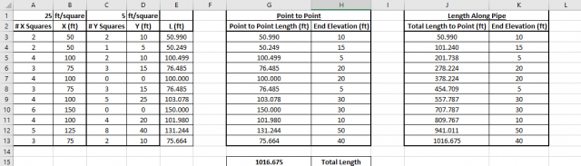
Table 2 – Intermediate pipe length segments defined. Options to copy and paste Intermediate Elevation data for “Point to Point” option or “Length Along Pipe” option.
Once you’ve pasted the appropriate data depending on the option you choose (either “Point to Point” or “Length Along Pipe”), you can click the “Show Graph” button and that will plot the elevation profile for you. Figure 5 shows the elevation profile of my model. As you can see, it matches the elevation changes defined by junctions originally in Figure 1.
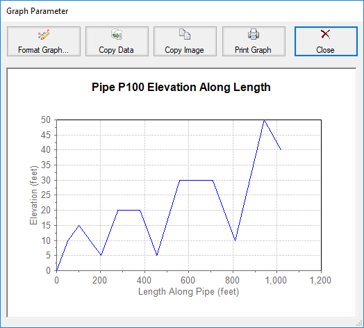
Figure 5 – Pipe Elevation Profile based upon Intermediate Pipe Elevation Data.
Let’s say you’ve detailed the Intermediate Pipe Elevations for your single pipe, and then later you find out there is a component in the pipeline that needs to be explicitly modeled. For example, a control valve exists in the horizontal segment of pipe between the 7th and 8th intermediate points, like in Figure 6.
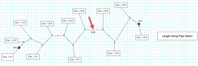
Figure 6 – Future location of Control Valve, located between the 30 ft (9.1 m) Intermediate Elevation Points.
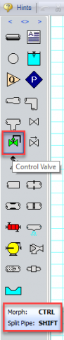
Figure 7 – Hot key ToolTips for Control Valve.
Well, no need to worry! You do NOT need to break any pipe and junction connections, drag a new junction, and draw a new pipe. No need to re-specify the lengths either. There is a much easier way…Whenever you hover over any junction on the Toolbox, a Tool Tip appears with hot key options to either morph a junction, or to split the pipe. Figure 7 (at the right) shows the hot keys for a Control Valve. So, what we will do is we are going to hold the Shift key down while dragging the Control Valve onto the Workspace and lay it on top of the pipe right where the arrow is pointing in Figure 6.
In previous versions when you split a pipe, the pipe would automatically be split in half. You would then have to manually go into each pipe and update the lengths.
Now, there is a brand-new feature in the latest versions that gives you much better control over the split ratio as well as which pipe you would like to move any minor fittings and losses onto! Figure 8 shows how I will be splitting the pipe between the two points at 30-foot (9.1 meter) elevation. I can easily control EXACTLY where the Control Valve junction will go. The greatest advantage is that this will also correctly update which intermediate elevation points need to go with which pipe. No need to re-work any intermediate pipe elevations at all, this will be done for you.
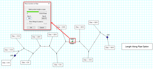
Figure 8 – Splitting the pipe with a Control Valve. New upstream and downstream pipe length controlled by scroll bar or directly entering length of new upstream pipe.
Figure 9 shows the system after splitting the pipe. There are now two pipes on the Workspace in this system and the Intermediate Elevation Points were automatically re-assigned accordingly.
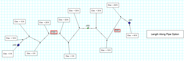
Figure 9 – Pipeline wither Intermediate Elevation Points – after pipe has been split.
Overall, using the Intermediate Pipe Elevation feature is an incredibly easy way to account for all your elevation changes without using extra junctions. The Intermediate Pipe Elevation data can easily be copied and pasted from a spreadsheet or imported from a text file. The Split Pipe feature allows you to quickly add in new junctions to your model without having to break pipe connections with drawing new pipes.
Lastly, there are two options now that make it even easier to assign Intermediate Pipe Elevations. Which one should you use? Well, the “Point to Point” option is much easier to specify from the get-go and does not require you to calculate the cumulative length along the pipe. However, using the “Length Along Pipe” option makes it easier to correctly specify where the new junction needs to be placed when specifying the split ratio. Ultimately, regardless of which option you choose, copying and pasting the data from Excel is the easiest way to go rather than typing in the points manually.
For your convenience, the Model used in this example can be found at the bottom of my blog here. AFT is always happy to work with you and address specific questions or help you troubleshoot your models. Please contact us at info@aft.com or (719) 686-1000.
Try a *FREE* Demo!

See more from Applied Flow Technology!